
I use the section-class plotting method in the oce package a lot. It’s one of the examples I really like showing to new oceanographic users of R and oce, to see the power in making quick plots from potentially very complicated data sets. A canonical example is to use the built-in data(section) dataset:
library(oce)
data(section)
plot(section, which='temperature')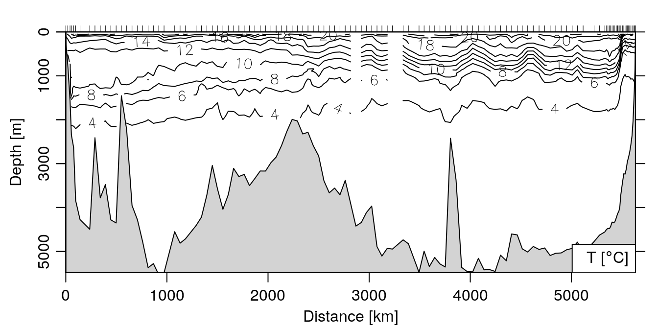
Note the grey bottom profile that is automatically overlaid on the plot – the values for those points come from the individual stations in the section object, from the waterDepth metadata item in each of the stations in the section. The values can be extracted to a vector with our trusty friend lapply1:
depth <- unlist(lapply(section[['station']], function(x) x[['waterDepth']]))
distance <- unique(section[['distance']])
plot(distance, depth, type='l')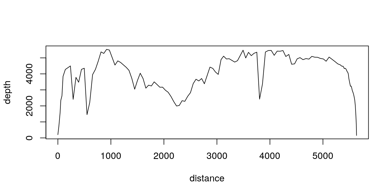
However, many CTD datasets don’t automatically include the water depth at the station, and even if they do the large spacing between stations may make the bottom look clunky.
Using the marmap package to add a high res bottom profile
To add a nicer looking profile to the bottom, we can take advantage of the awesome marmap package, which can download bathymetric data from NOAA.
To add a nice looking bottom profile to our section plot, we can use the getNOAA.bathy() and get.depth() functions. Note the resolution=1 argument, which downloads the highest resolution data available from NOAA (1 minute resolution), and the keep=TRUE argument, which saves a local copy of the data to prevent re-downloading every time the script is re-run (note that at 1 minute resolution the csv file obtained below is 29 MB):
library(marmap)
lon <- section[["longitude", "byStation"]]
lat <- section[["latitude", "byStation"]]
lon1 <- min(lon) - 0.5
lon2 <- max(lon) + 0.5
lat1 <- min(lat) - 0.5
lat2 <- max(lat) + 0.5

## get the bathy matrix -- 29 MB file
b <- getNOAA.bathy(lon1, lon2, lat1, lat2, resolution=1, keep=TRUE)
plot(section, which="temperature", showBottom=FALSE)
loni <- seq(min(lon), max(lon), 0.1)
lati <- approx(lon, lat, loni, rule=2)$y
dist <- rev(geodDist(loni, lati, alongPath=TRUE))
bottom <- get.depth(b, x=loni, y=lati, locator=FALSE)
polygon(c(dist, min(dist), max(dist)), c(-bottom$depth, 10000, 10000), col='grey')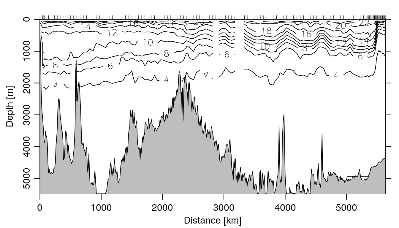
Nice!