Bootstrapping uncertainties with the boot package

Fitting models, with uncertainties!

Recently I found myself needing to estimate both the slope and x-intercept for a linear regression. Turns out it’s pretty easy for the slope, since it’s one of the directly estimated parameters from the regression (using the lm() function), but it wasn’t as clear how to get the uncertainty for the x-intercept. In steps the boot package, which is a nice interface for doing bootstrap estimation in R. I won’t get into the fundamentals of what bootstrapping involves here (the linked wikipedia article is a great start).

Ok, first, a toy example (which isn’t all that different from my real research problem). We make some data following a linear relationship (with noise):

library(boot)
x <- 0:20
set.seed(123) # for reproducibility
y <- x + rnorm(x)
plot(x, y)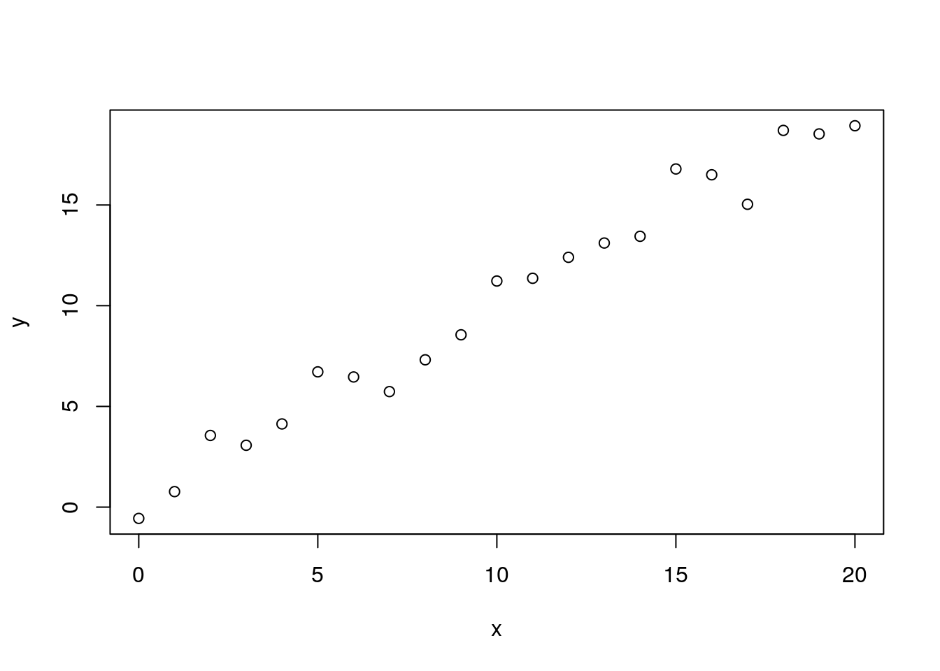

We can easily fit a linear model to this using the lm() function, and display the results with the summary() function:

m <- lm(y ~ x)
plot(x, y)
abline(m)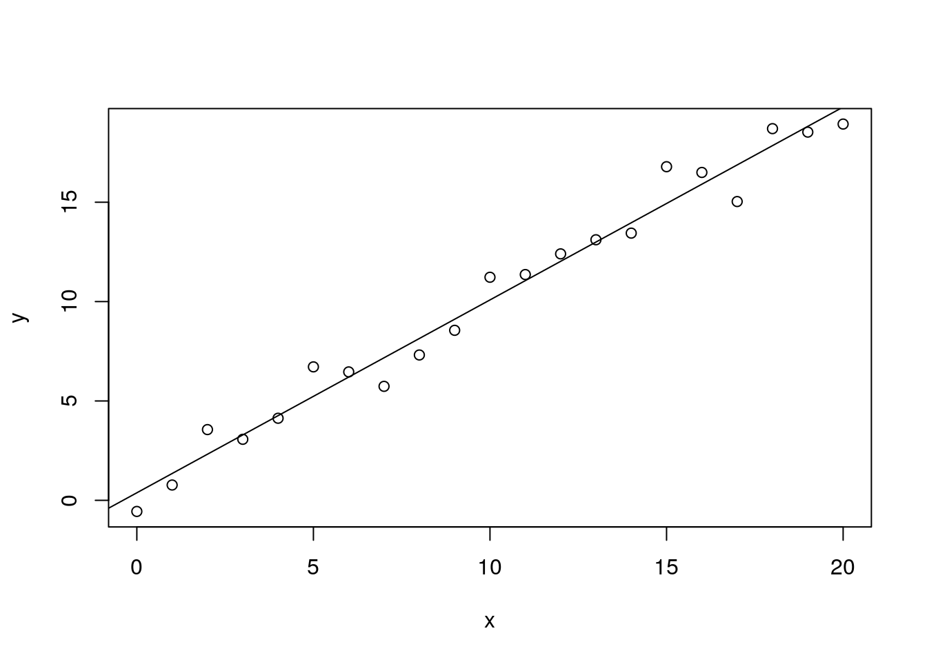

summary(m)

## 
## Call:
## lm(formula = y ~ x)
## 
## Residuals:
##     Min      1Q  Median      3Q     Max 
## -1.8437 -0.5803 -0.1321  0.5912  1.8507 
## 
## Coefficients:
##             Estimate Std. Error t value Pr(>|t|)    
## (Intercept)  0.37967    0.41791   0.909    0.375    
## x            0.97044    0.03575  27.147   <2e-16 ***
## ---
## Signif. codes:  0 '***' 0.001 '**' 0.01 '*' 0.05 '.' 0.1 ' ' 1
## 
## Residual standard error: 0.992 on 19 degrees of freedom
## Multiple R-squared:  0.9749, Adjusted R-squared:  0.9735 
## F-statistic:   737 on 1 and 19 DF,  p-value: < 2.2e-16

I love lm(). It’s so easy to use, and there’s so much information attached to the result that it’s hard not to feel like you’re a real statistician (even if you’re an imposter like me). Check out the neat little table, showing the estimates of the y-intercept and slope, along with their standard errors, t values, and p values.

So how to get the error on the x-intercept? Well, one way might be to propagate the slope and y-intercept uncertainties through a rearrangement of the \(y = a + bx\) equation, but for anything even a little complicated this would be a pain. Let’s do it instead with the boot package.

We need to create a function that takes the data (as the first argument), with the second argument being an index that can be used by the boot() function to run the function with a subset of the data. Let’s demonstrate first by writing a function to calculate the slope, and see how the bootstrapped statistics compare with what comes straight from lm():

slope <- function(d, ind) {
    m <- lm(y ~ x, data=d[ind,])
    coef(m)[[2]]
}
slope_bs <- boot(data.frame(x, y), slope, 999)
slope_bs

## 
## ORDINARY NONPARAMETRIC BOOTSTRAP
## 
## 
## Call:
## boot(data = data.frame(x, y), statistic = slope, R = 999)
## 
## 
## Bootstrap Statistics :
##      original     bias    std. error
## t1* 0.9704362 0.00127172  0.03634102

The bootstrap estimate decided (using 999 subsampled replicates) that the value of the slope should be 0.970436155978, while that straight from the linear regression gave 0.970436155978 (i.e. exactly the same!). Interestingly the standard error is slightly higher than from lm(). My guess is that would get closer to the real value with more replicates.

Ok, now to do it for the x-intercept, we just supply a new function:

xint <- function(d, ind) {
    m <- lm(y ~ x, data=d[ind,])
    -coef(m)[[1]]/coef(m)[[2]] # xint = -a/b
}
xint_bs <- boot(data.frame(x, y), xint, 999)
xint_bs

## 
## ORDINARY NONPARAMETRIC BOOTSTRAP
## 
## 
## Call:
## boot(data = data.frame(x, y), statistic = xint, R = 999)
## 
## 
## Bootstrap Statistics :
##       original       bias    std. error
## t1* -0.3912359 -0.003184903   0.4381748

So the bootstrap estimate of the x-intercept is -0.3912359 \(\pm\) 0.4381748