
Introduction
I’ve been working on a project related to measurement errors due to thermal boundary layers as a sensor moves through oceanic vertical temperature gradients. It’s a very similar problem to that discussed by Lueck (1990)1, Lueck and Picklo (1990)2, and Morison et al (1994)3 (except applied to an RBR external-field inductive CTD), however I am trying to extend the theory to make the model of the error a little more accurate.
To do this, I need to make use of the Blasius solution for the structure of a laminar boundary layer. Solved originally in 1908, the problem is interesting because there isn’t an easy analytical solution, and therefore it has to be solved numerically. This blog post is the culmination of my work to understand the problem, it’s solution (in R), and how to define a simple analytical approximation that is suitable for the boundary-layer structure needed for the error model.
The Blasius equation for a laminar boundary layer on a flat plat (at zero incidence)

Figure 1: Laminar boundary layer on a flat plate
The Blasius equation is derived from the frictional steady state \(x\) momentum equation, neglecting pressure gradients, in combination with the standard two dimensional continuity equation:
\[ u \frac{\partial u}{\partial x} + v \frac{\partial u}{\partial y} = \nu \frac{\partial^2 u}{\partial y^2} \]
\[ \frac{\partial u}{\partial x} + \frac{\partial v}{\partial y} = 0 \]
For the problem setup, we consider uniform “free stream” flow with speed \(U_\infty\) and we seek to find the profile of velocity \(U(y)\) within the boundary layer. As discussed by Blasius, since the system has no preferred length a good assumption is that the velocity profiles at varying distances from the leading edge all have the same form, and can be made identical by an appropriate scaling for \(u\) and \(y\).
Scaling
To scale the variables we define a new vertical coordinate \(\eta = y/\delta\), where \(\delta\) is the approximate boundary layer thickness, so that:
\[ \eta = y \sqrt{\frac{U_\infty}{\nu x}} \]
The continuity equation can be integrated by introducting a stream function \(\psi\), which can be written as:
\[ \psi = \sqrt{\nu x U_\infty} \,\, f(\eta), \]
where \(f(\eta)\) is the dimensionless stream function.
The \(u\) velocity components can be written as
\[ u = \frac{\partial \psi}{\partial y} = \frac{\partial \psi}{\partial \eta} \frac{\partial \eta}{\partial y} = U_\infty f'(\eta)\]
where the prime represents differentiation wrt to \(\eta\). Similarly the \(v\) component is
\[ v = - \frac{\partial \psi}{\partial x} = \frac{1}{2} \sqrt{\frac{\nu U_\infty}{x}} (\eta \, f' - f)\]
Other required terms can be further derived, including \(\partial u/\partial x\), \(\partial u/\partial y\), and \(\partial^2 u/\partial y^2\):
\[ \frac{\partial u}{\partial x} = U_\infty \, f''(\eta) \left(-\frac{1}{2} \right) \frac{\eta}{x} = -\frac{U_\infty \eta}{2 x} \, f''(\eta) \]
\[ \frac{\partial u}{\partial y} = U_\infty \,f''(\eta) \frac{\partial \eta}{\partial y} = U_\infty \sqrt{\frac{U_ \infty}{\nu x}} \, f''(\eta) \]
\[ \frac{\partial^2 u}{\partial y^2} = U_\infty \sqrt{\frac{U_\infty}{\nu x}} \left( f'''(\eta) \sqrt{\frac{U_\infty}{\nu x}} \right) = \frac{U_\infty^2}{\nu x} \, f'''(\eta) \]
Substituting all terms into the \(x\) momentum equation gives
\[ -\frac{U_\infty^2}{2 x} \eta \, f' \, f'' + \frac{U_\infty^2}{2 x} (\eta \, f' - f) \, f'' = \frac{U_\infty^2}{x} \, f'''\]
which can be simplified to
\[ f \, f'' + 2\, f''' = 0 \]
or, to be consistent with the later numerical approach,
\[ f''' + \frac{1}{2} \, f \, f'' = 0 \]
Boundary conditions
The boundary conditions correspond to
\[ f(\eta=0) = 0, \,\,\, f'(\eta=0) = 0 \]
and
\[ f'(\eta = \infty) = 1 \]
The latter BC describes the fact that at large \(y\) the value must approach the free stream velocity \(U_\infty\).
The resulting differential equation is both nonlinear and of the third order, thus the 3 BCs are sufficient to determine the solution. However, there is no exact analytical solution, and must therefore be solved either approximately (e.g. by a series expansion method as done by Blasius) or numerically (as done by Howarth in 19384). One possible numerical approach will be explored in the next section.
Numerical solution
When working with differential equations in R, I am often amazed by just how powerful the deSolve package is. Of course, it’s basically just an R wrapper around a lot of long-standing and well-testing numerical solvers, but as a scientist it sometimes feels like having a secret superpower. I’ve used it for several projects over the last few years to great success.
That being said, I do sometimes find the interface (and the variety of methods and options) somewhat overwhelming. So for this example, I ended up going down a slightly different road; creating my own DE solver code. I’m sure that with some more squinting and googling I could figure out how to do it with deSolve but actually I ending up being pleasantly surprised by just how simple it ended up being to roll my own solver for this problem.
Classic textbooks (e.g. Schlicting5) outline that the typical approach to solve the Blasius problem is to use a Runge-Kutta method. A further refinement over the straight-up RK4 method, which I’ll show below, is that one of the parameters required to determine the solution is unknown. To get around this, a common method known as the “shooting method” is used, where the parameter is guessed and the solution found, which is then compared with the boundary conditions. Refinements to the guess that bring the solution in line with the boundary condition can then be made, until the BC is satisfied (to within some tolerance).
4th order Runge-Kutta scheme6
The classic Runge-Kutta method for numerically solving a differential equation involves creating a weighted average of slopes and using that combined with the previous value to estimate each new value (see Figure 2). When run from an initial condition, this can be used to solve the differential equation. Classically this is thought of as an integration in time (in oceanography, I hear the terms “Runge-Kutta” most often when listening to talks by modelers who use their model velocity output to simulate drifters), but it can be used for any generic DE system.
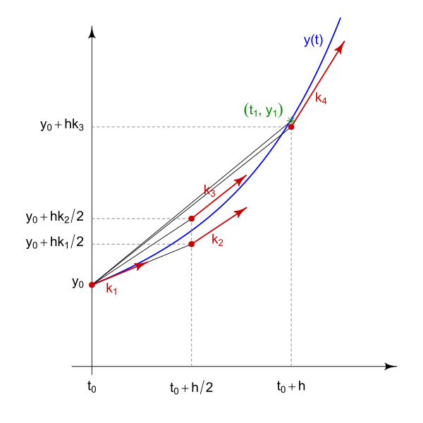
Figure 2: Runge-Kutta method, from Wikipedia
To implement the RK4 algorithm, we create a function that implements the weighted average algorithm based on the input function fz\(=f(z)\), it’s first derivative fp\(=f'(z)\), and the step size dz.
rk4 <- function(fz, fp, dz) {
    k1 <- fp(fz)
    k2 <- fp(fz+dz/2*k1)
    k3 <- fp(fz+dz/2*k2)
    k4 <- fp(fz+dz*k3)
    return(fz + dz/6*(k1+2*k2+2*k3+k4))
}
In order to apply the RK4 method to the Blasius equation, which is a third-order DE, we have to replace it with three first-order DEs, e.g.
\[ F' = G \]
\[ G' = H \]
\[ H' = F''' = -\frac{1}{2} F H \]
To do this, we create a function for the first derivatives so that we can simultaneously solve the coupled system:
fp <- function(f) {
    return(c(f[2], f[3], -0.5*f[1]*f[3]))
}
We can use the initial conditions and set up the arrays for the solution, according to \(F(0) = 0\), \(F'(0) = G(0) = 0\), and \(F'(\infty) = G(\infty) = 1\). However, we also need a condition for \(F''(0) = H(0)\), which is unknown. This is where the shooting method comes in; we make a guess for \(H(0)\), solve the system, and check whether the far-field boundary condition \(F'(\infty) = 1\) is satisfied. \(H(0)\) can then be adjusted to achieve the far-field condition.
Choosing a random value of \(H(0) = 0.5\), the solution produces:
H0 <- 0.5

dz <- 0.05
Z <- 10
N <- Z/dz
z <- seq(0, Z-dz, dz)
F <- G <- H <- rep(0, N)
H[1] <- H0
for (i in 1:(N-1)) {
    fz <- c(F[i], G[i], H[i])
    fz2 <- rk4(fz, fp, dz)
    F[i+1] <- fz2[1]
    G[i+1] <- fz2[2]
    H[i+1] <- fz2[3]
}
plot(z, G)
grid()
abline(h=1)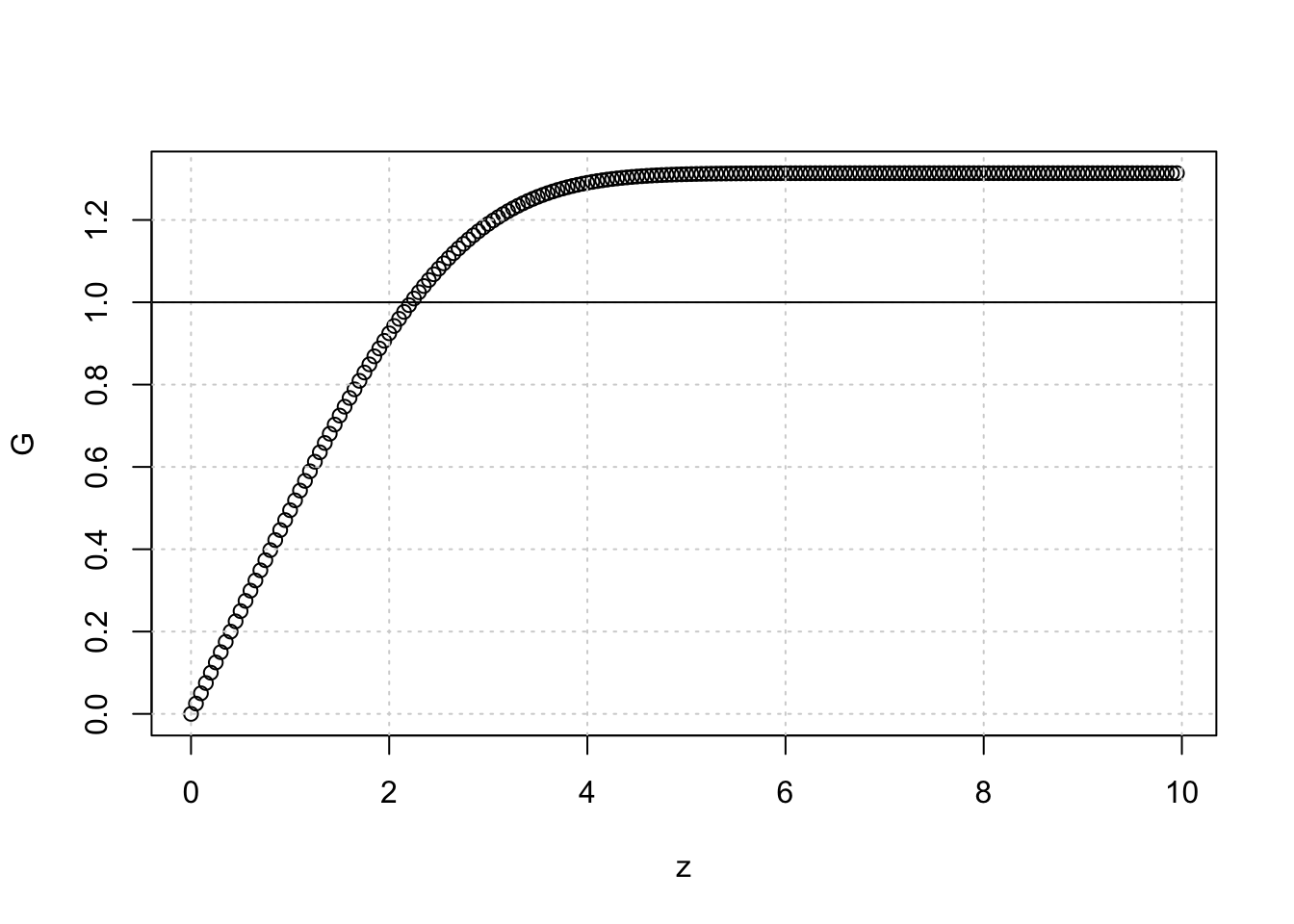
Remember that \(G(\infty) = 1\), so it’s clear that our guess for \(H(0)\) is too high. Trial and error suggests that an appropriate value is \(H(0) \sim 0.33\), however we can easily do better than this by wrapping the solver in a loop and iterating based on an error tolerance:
Hmin <- 0
Hmax <- 1
err <- 1
counter <- 1
dz <- 0.05
Z <- 10
N <- Z/dz
z <- seq(0, Z-dz, dz)
HH <- NULL
while (abs(err) > 1e-6) {
    H0 <- (Hmin + Hmax)/2
    HH[counter] <- H0
    F <- G <- H <- rep(0, N)
    H[1] <- H0
    for (i in 1:(N-1)) {
        fz <- c(F[i], G[i], H[i])
        fz2 <- rk4(fz, fp, dz)
        F[i+1] <- fz2[1]
        G[i+1] <- fz2[2]
        H[i+1] <- fz2[3]
    }
    err <- tail(G, 1) - 1
    if (err < 0) Hmin <- H0 else Hmax <- H0
    ## plot(z, G)
    ## abline(h=1)
    counter <- counter + 1
}

par(mfrow=c(2, 1), mar=c(3, 3, 1, 1), mgp=c(1.5, 0.5, 0))
plot(z, G); grid()
plot(HH, type='l', ylim=c(0, 1), xlab='Iteration', ylab='H0 guess'); grid()
mtext(paste0('H0 = ', format(tail(HH, 1), digits=6)), side=3, line=-2, adj=1, cex=2)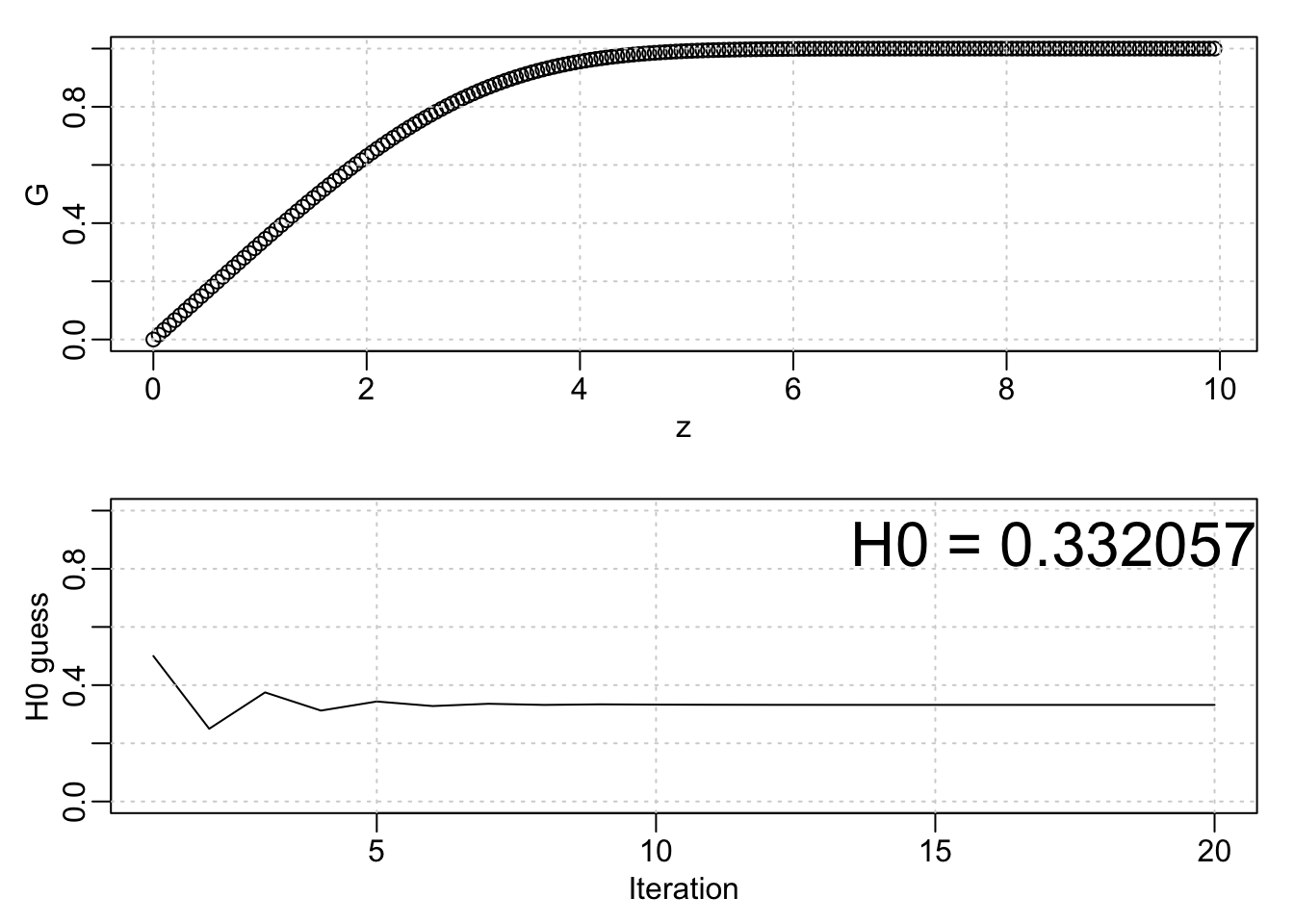
Analytical approximation to the full solution
The approach above gives us the true solution to the Blasius equation – however, because it has no analytical form it is not conducive to using for further (theoretical or numerical) analysis. One solution would be to fit a functional form that gives a good approximation.
One such form can be found here7, which posits an analytical form for the Blasius solution and then determines the best parameters to match. The proposed expression takes the form:
\[ u(\eta) = f'(\eta) = \left( \tanh \left[ (a \eta)^n \right] \right)^{1/n} \]
The optimal values for the parameters \(a\) and \(n\) are 0.33206 and 3/2 (note the similarity between the value of \(a\) and \(H(0)\) above). Comparing the analytical form with the true solution gives:
fp_approx <- function(eta, a=0.33206, n=3/2) {
    (tanh( (a*eta)^n ))^(1/n)
}

par(mfrow=c(2, 1), mar=c(3, 3, 1, 1), mgp=c(1.5, 0.5, 0))
plot(z, G, type='l', lwd=2, ylab=expression(u*"("*eta*")")); grid()
legend('bottomright', c('Full solution', 'Approximation'), lty=1, lwd=2, col=1:2)
lines(z, fp_approx(z), lwd=2, col=2)
plot(z, 100*(fp_approx(z) - G), type='l', lwd=2, ylab='Percent difference'); grid()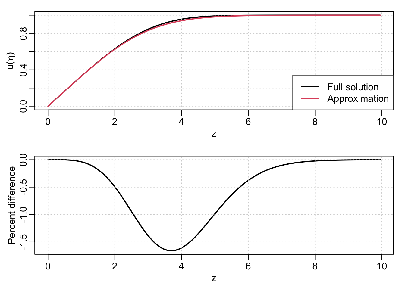
References
Lueck, R. G. Thermal inertia of conductivity cells: Theory. Journal of Atmospheric and Oceanic Technology 7, 741–755 (1990).↩︎
Lueck, R. G. & Picklo, J. J. Thermal Inertia of Conductivity Cells: Observations with a Sea-Bird Cell. J. Atmos. Oceanic Technol. 7, 756–768 (1990).↩︎
Morison, J., Andersen, R., Larson, N., D’Asaro, E. & Boyd, T. The Correction for Thermal-Lag Effects in Sea-Bird CTD Data. J. Atmos. Oceanic Technol. 11, 1151–1164 (1994).↩︎
Howarth, L. On the solution of the laminar boundary layer equations. Proceedings of the Royal Society of London. Series A-Mathematical and Physical Sciences 164, 33 (1938).↩︎
Schlichting H, Kestin J. Boundary layer theory. New York: McGraw-Hill; 1961.↩︎
Inspiration for much of this section came from the following notebook post: https://notebook.community/ultiyuan/test0/lessons/Blasius↩︎
Savaş, Ö. An approximate compact analytical expression for the Blasius velocity profile. Communications in Nonlinear Science and Numerical Simulation 17, 3772–3775 (2012).↩︎