RBR-equipped Alamo float in Alex Honnold's 'Arctic Ascent'

2024-06-09 in OCEANOGRAPHY
rbr alamo argo profiling omg ctd
4 min read

Introduction

An RBR Alamo float, freshly dropped into a Greenlandic fjord

The other day, for “Friday Family Movie and Pizza Night”, we decided to throw on Arctic Ascent with Alex Honnold. Having watched his previous film, Free Solo a couple years ago, I knew that it was going to be about climbing. But what I didn’t know was that for the expedition to an unclimbed sea cliff in Greenland, he brought along glaciologist Heidi Sevestre so that they could take some unique data along the way.

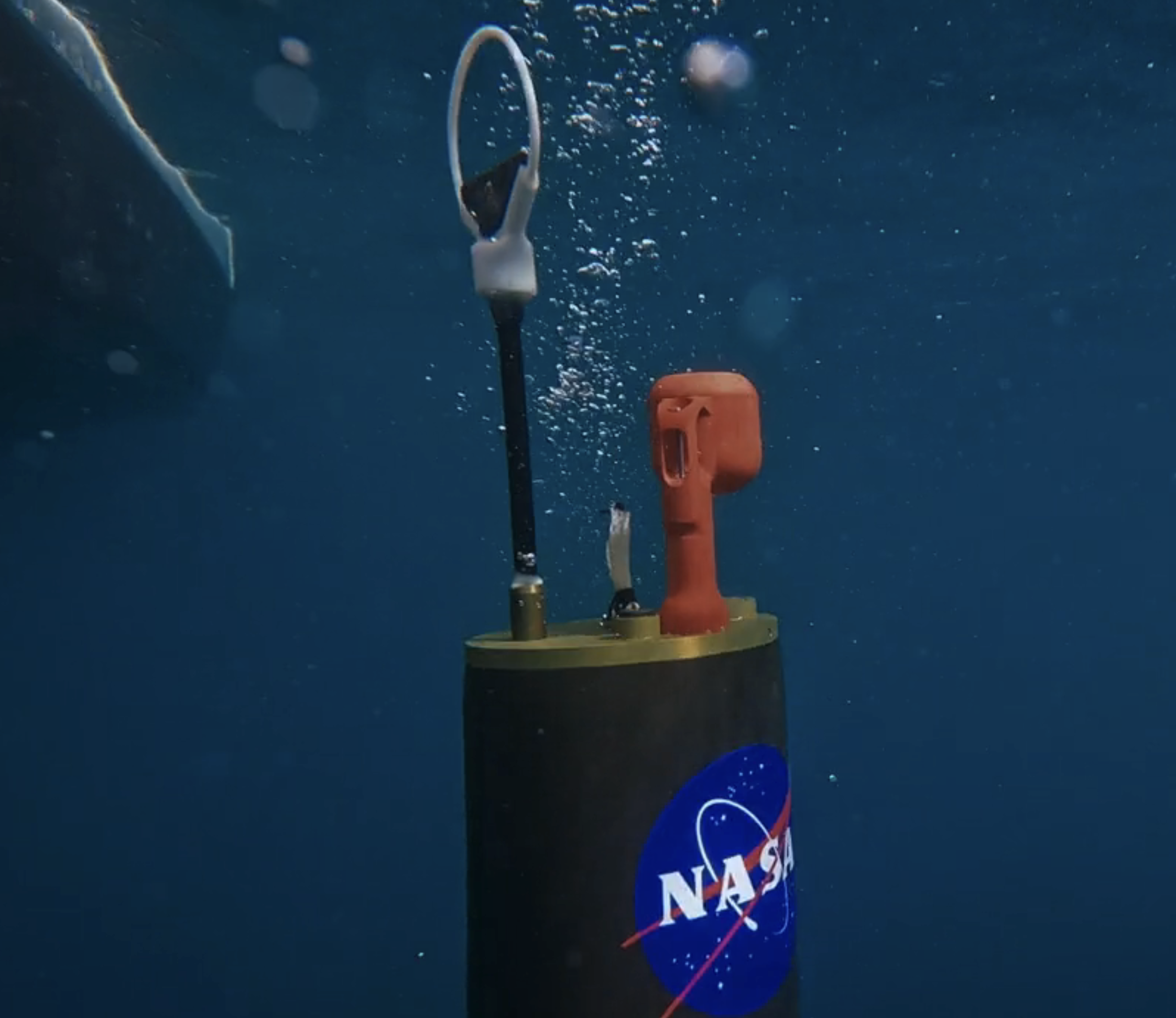
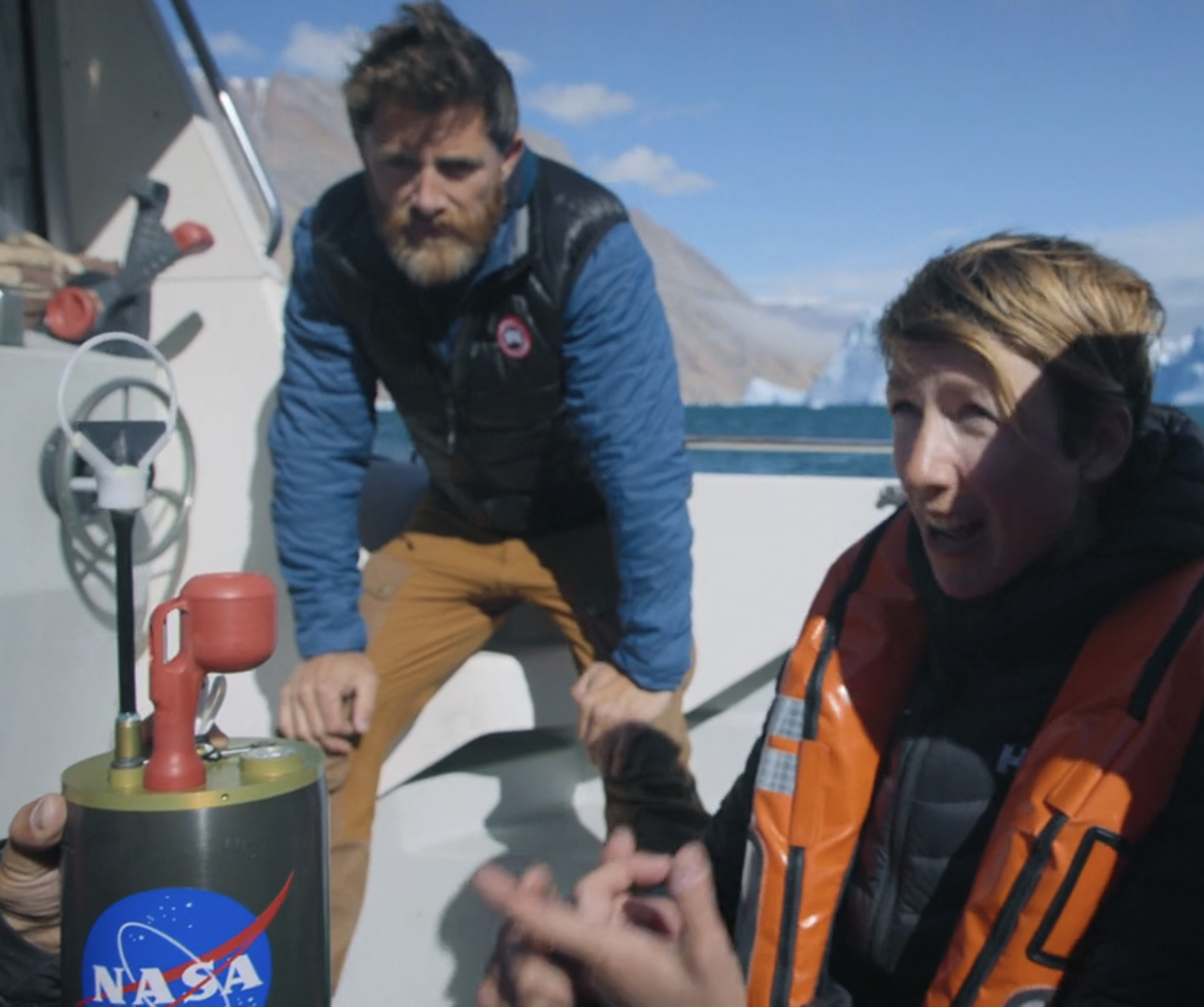
Much to my surprise, in episode 2, after getting picked up along the coastline in a boat by their team, they proceeded to unpack and deploy an RBRargo-equipped MRV Alamo float to deploy inside the fjord. My family rolled their eyes at me, as I shouted “That’s an argo float! And it’s got an RBR CTD on it!”¹.

The float is unboxed

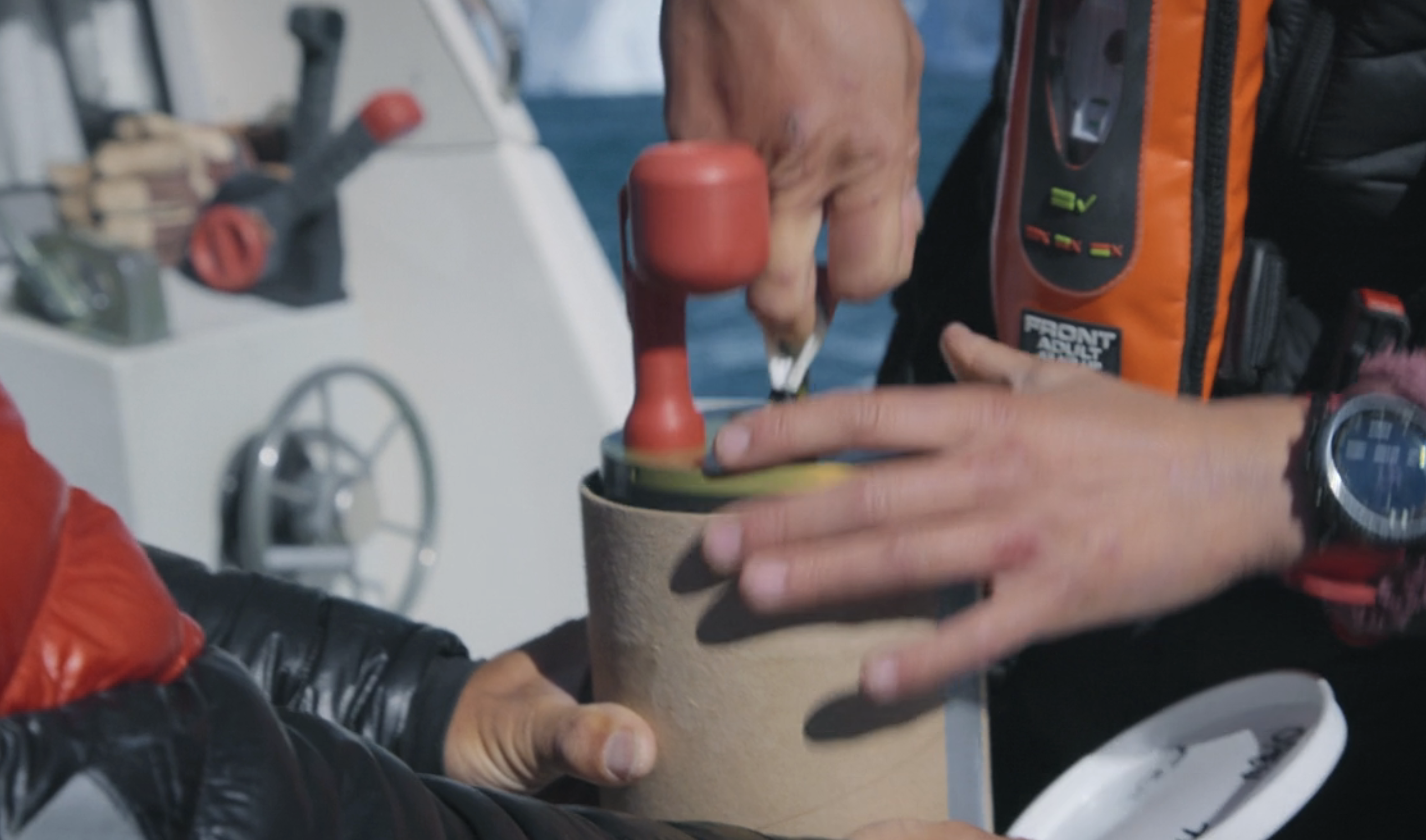
The float was contributed to the expedition by the Oceans Melting Greenland (i.e. “OMG”) project, a huge NASA-led project that saw hundreds of expendable floats/sensors dropped all around Greenland over a number of years to attempt to quantify ocean properties on a scale not previously possible. In the episode, Alex says that they’re float is number 9317, which gave me enough information to start digging around to see if I could find the data (cue family eyeroll again).

Heidi explains how the float works, while Aldo looks on

Data

After checking the usual “Argo” channels, and not finding anything in Greenlandic fjords, I started googling for more specific terms related to the OMG project. That eventually led me to the following NASA/JPL page:

https://podaac.jpl.nasa.gov/dataset/OMG_L1_FLOAT_ALAMO

Clicking through to “Data Access” and then on the “Browse” earthdata link, got me eventually to this page, which listed all the days in August that there was Alamo data for:

https://cmr.earthdata.nasa.gov/virtual-directory/collections/C2491772150-POCLOUD/temporal/2022/08

I couldn’t see an obvious way to hack the url to download everything, so I just took the 3 minutes to click through each of the days and manually download the text file versions for float 9317, e.g.

https://archive.podaac.earthdata.nasa.gov/podaac-ops-cumulus-public/OMG_L1_FLOAT_ALAMO/OMG_Alamo_F9317_Dive_000.20220806T165559_text.txt

Reading the data

Let’s see what we’ve got for data, and try and read it into R as oce/ctd objects

library(oce)

## Loading required package: gsw

files <- dir('rbr_alamo_data', pattern='*.txt')
files

##  [1] "OMG_Alamo_F9317_Dive_000.20220806T165559_text.txt"
##  [2] "OMG_Alamo_F9317_Dive_001.20220806T180135_text.txt"
##  [3] "OMG_Alamo_F9317_Dive_003.20220807T044632_text.txt"
##  [4] "OMG_Alamo_F9317_Dive_004.20220807T102605_text.txt"
##  [5] "OMG_Alamo_F9317_Dive_005.20220807T160759_text.txt"
##  [6] "OMG_Alamo_F9317_Dive_006.20220807T233322_text.txt"
##  [7] "OMG_Alamo_F9317_Dive_007.20220808T094558_text.txt"
##  [8] "OMG_Alamo_F9317_Dive_008.20220808T151420_text.txt"
##  [9] "OMG_Alamo_F9317_Dive_009.20220808T204256_text.txt"
## [10] "OMG_Alamo_F9317_Dive_010.20220809T020036_text.txt"
## [11] "OMG_Alamo_F9317_Dive_011.20220809T072018_text.txt"
## [12] "OMG_Alamo_F9317_Dive_012.20220809T134056_text.txt"
## [13] "OMG_Alamo_F9317_Dive_013.20220809T195710_text.txt"
## [14] "OMG_Alamo_F9317_Dive_014.20220810T023743_text.txt"
## [15] "OMG_Alamo_F9317_Dive_015.20220810T093639_text.txt"
## [16] "OMG_Alamo_F9317_Dive_018.20220813T055153_text.txt"
## [17] "OMG_Alamo_F9317_Dive_019.20220814T122944_text.txt"
## [18] "OMG_Alamo_F9317_Dive_020.20220814T193430_text.txt"
## [19] "OMG_Alamo_F9317_Dive_021.20220815T025606_text.txt"
## [20] "OMG_Alamo_F9317_Dive_022.20220818T031945_text.txt"
## [21] "OMG_Alamo_F9317_Dive_023.20220818T103751_text.txt"
## [22] "OMG_Alamo_F9317_Dive_024.20220821T105746_text.txt"
## [23] "OMG_Alamo_F9317_Dive_025.20220824T111510_text.txt"
## [24] "OMG_Alamo_F9317_Dive_026.20220827T113132_text.txt"
## [25] "OMG_Alamo_F9317_Dive_027.20220828T114858_text.txt"

So, 25 files in all, as plain text. Turns out they’re not “simple” csvs or something, so I need to hack together a file parser to read the data that I want (the ascent data), as well as any relevant metadata (time, longitude, latitude). The reading function looks like:

read_omg_alamo <- function(file) {
    require(oce)
    l <- readLines(file)
    time <- l[grep('fix time', l)] |> gsub('fix time: ', '', x=_) |> as.POSIXct(tz='UTC')
    longitude <- l[grep('longitude', l)] |> gsub('longitude: ', '', x=_) |> as.numeric()
    latitude <- l[grep('latitude', l)] |> gsub('latitude: ', '', x=_) |> as.numeric()
    start <- grep('ascending', l) + 4
    end <- tail(grep('unbinned', l), 1) - 3
    txt <- l[start:end]
    txt2 <- unlist(lapply(txt, function(x) gsub('║', '', x)))
    d <- read.delim(text=txt2, header=FALSE, sep='')
    d$V2 <- d$V4 <- d$V6 <- NULL
    names(d) <- c('pressure', 'temperature', 'salinity', 'temperatureConductivity')
    ctd <- as.ctd(d)
    ctd <- oceSetMetadata(ctd, 'startTime', time[1])
    ctd <- oceSetMetadata(ctd, 'endTime', time[2])
    ctd <- oceSetMetadata(ctd, 'longitude', longitude[2])
    ctd <- oceSetMetadata(ctd, 'latitude', latitude[2])
    ctd <- oceSetMetadata(ctd, 'startLongitude', longitude[1])
    ctd <- oceSetMetadata(ctd, 'startLatitude', latitude[1])
    return(ctd)
}

Now I can rip through the list of files, reading them into a list of ctd objects.

files <- dir('rbr_alamo_data', pattern='*.txt', full.names = TRUE)[-1] # drop the first one
ctd <- lapply(files, read_omg_alamo)  # creates a list of ctd objects
sec <- as.section(ctd)  # create a section object

## Warning in as.section(ctd): estimated waterDepth as max(pressure) for CTDs
## numbered 1:24

plot(sec, which='map', span=100)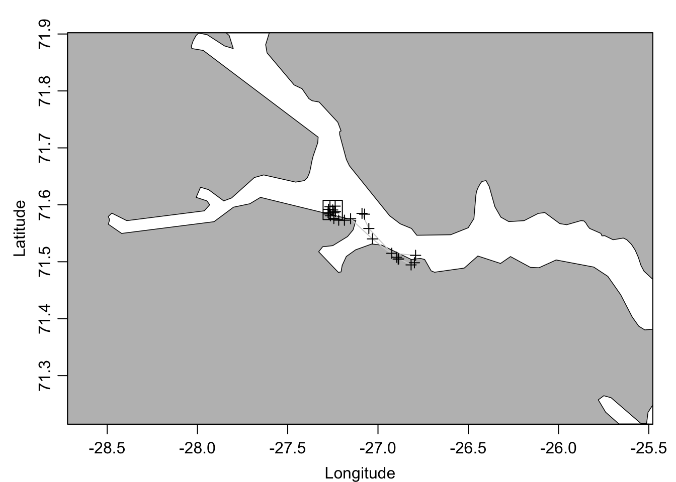

We can make a TS plot of the profiles:

plotTS(sec)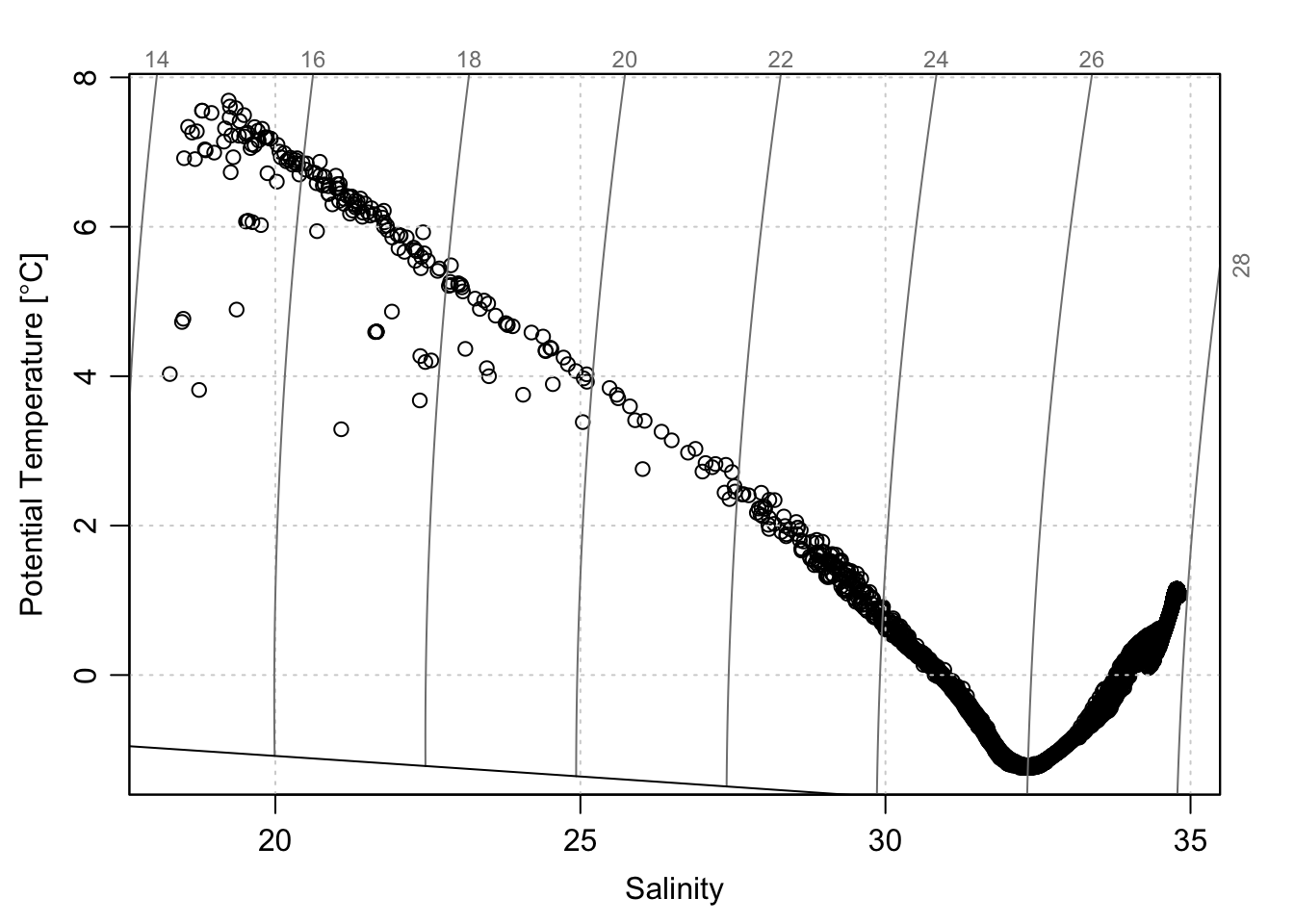

And we can look at the T and S profiles, first for the entire depth covered by the float (approximately 1000m), and then zoomed in on the top 100m:

par(mfrow=c(1, 2))
plotProfile(ctd[[1]], xtype='temperature', lty=0, Tlim=c(-1, 8))
jnk <- lapply(ctd, plotProfile, xtype='temperature', add=TRUE)
plotProfile(ctd[[1]], xtype='salinity', lty=0, Slim=c(17, 35))
jnk <- lapply(ctd, plotProfile, xtype='salinity', add=TRUE)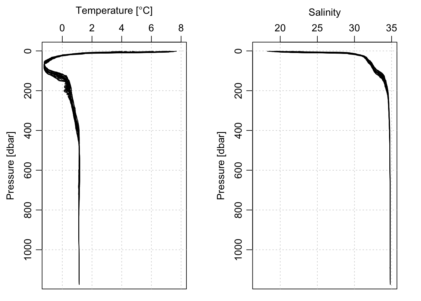

plotProfile(ctd[[1]], xtype='temperature', lty=0, Tlim=c(-1, 8), plim=c(100, 0))
jnk <- lapply(ctd, plotProfile, xtype='temperature', add=TRUE)
plotProfile(ctd[[1]], xtype='salinity', lty=0, Slim=c(17, 35), plim=c(100, 0))
jnk <- lapply(ctd, plotProfile, xtype='salinity', add=TRUE)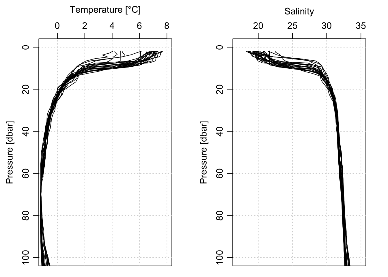

While I generally consider myself an expert in CTD identification, I worked at RBR for a time between my postdoc and my current job with DFO. It was a formative 1.25 years, but one of the primary successes that I got to contribute to was a redesign of the conductivity cell into the “combined” conductivity/temperature cell that is now the ubiquitous RBRargo sensor. So, kind of easy for me to pick out :)↩︎

Introduction

Data

Reading the data

Related Articles