
In the spirit of continuing blog posts, this post follows from the last one: “Functions to model ocean interfaces”, in which I explored the “error function” as a nice model for a diffusive interface between two homogenous layers. Often I use these kinds of idealized interfaces for synthetic gradients, to simulate ocean sensor responses as they profile through a dynamic environment (see e.g. this recent paper by Martini et al.1). In fact, it was Dr. Kim Martini that inspired this deep dive in the first place.
Fitting data to models
In R, fitting data to a model is usually done using either the lm() (for linear models) or the nls() (for nonlinear models) functions. The first post in this series used nls() to fit a \(\tanh\) function to some real data from the Eastern North American continental shelf.
The nls() function allows you to specify your model using the “formula” syntax in R, that is, the call to do the fitting looks like this:
m <- nls(T ~ a + b*tanh((z-z0)/dz), start=list(a=3, b=1, z0=-10, dz=5))where the T ~ a + b*tanh((z-z0)/dz) part specifies the model in a “human readable” way that doesn’t require any fancy coding (the magic is in the ~ part of it, which TBH I never really have understood the details of).
The original data and \(\tanh\) fitting is as below:
library(oce)
ctd <- read.oce('D19002034.ODF')
## Warning in read.odf(file = file, columns = columns, exclude = exclude, debug =
## debug - : "CRAT_01" should be unitless, but the file states the unit as "S/m" so
## that is retained in the object metadata. This will likely cause problems. See ?
## read.odf for an example of rectifying this unit error.par(mfrow=c(1, 2))
plot(ctd, which=1, type='l')
plot(ctd, which=5)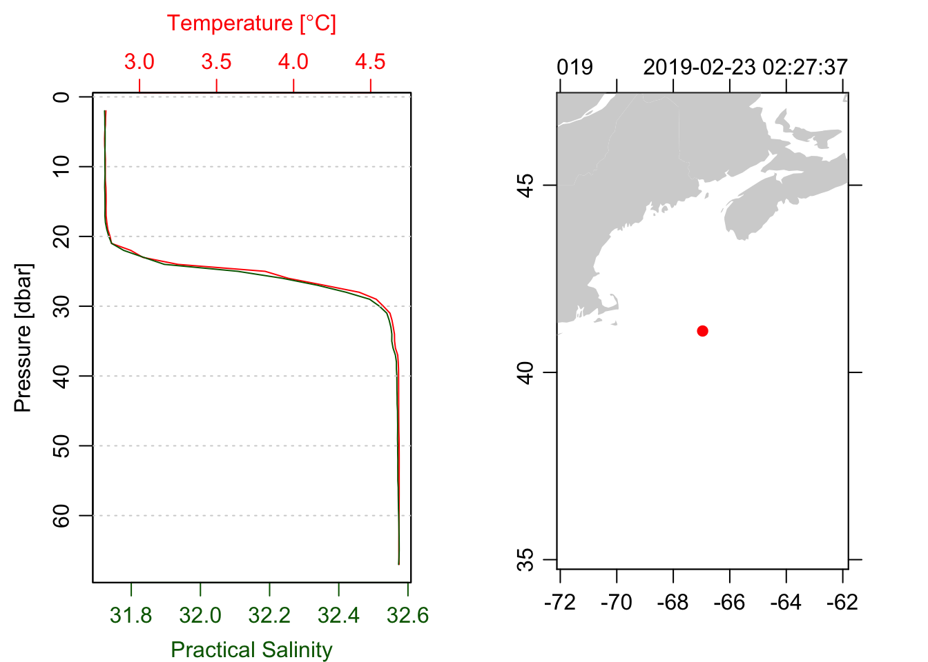
z <- -ctd[["depth"]]
T <- ctd[["temperature"]]
m <- nls(T ~ a + b*tanh(-(z-z0)/dz), start=list(a=3, b=1, z0=-10, dz=5))
m
## Nonlinear regression model
## model: T ~ a + b * tanh(-(z - z0)/dz)
## data: parent.frame()
## a b z0 dz
## 3.7251 0.9516 -25.0448 2.7647
## residual sum-of-squares: 0.05222
##
## Number of iterations to convergence: 10
## Achieved convergence tolerance: 4.496e-06What I hadn’t realized until I started looking into this, is that nls() can work with any R function, not just with analytical “formula”-style expressions. This is important for this post, because the nature of the analytical form of the “error function”:
\[ erf(z) = \frac{2}{\sqrt{\pi}} \int_0^z e^{-t^2}\,dt \]
which is an integral expression and therefore doesn’t work with the formula syntax in R.
However, in the last post we created a function that could be used to create an interface based on a number of parameters (e.g. top and bottom values, interface depth, and interface thickness):
interface <- function(z, zi, c1, c2, sigma=1) {
    gaussian <- function(z, sigma) 1/(sigma * sqrt(2*pi)) * exp(-1/2 * z^2/sigma^2)
    int <- Vectorize(function(z, sigma=1) integrate(gaussian, 0, z, sigma)$value)
    0.5*(c1 + c2) + (c1 - c2) * int(z - zi, sigma)
}
It turns out that we can feed this function straight into nls() to get a fit to determine the profile parameters:
mm <- nls(T ~ interface(z, zi, c1, c2, sigma), start=list(c1=3, c2=4.5, zi=-25, sigma=2))
mm
## Nonlinear regression model
## model: T ~ interface(z, zi, c1, c2, sigma)
## data: parent.frame()
## c1 c2 zi sigma
## 2.777 4.675 -25.060 2.327
## residual sum-of-squares: 0.05653
##
## Number of iterations to convergence: 5
## Achieved convergence tolerance: 5.908e-06The parameters aren’t exactly equivalent. In the \(\tanh\) model \(a\) represents the mean value and \(b\) represents the \(\Delta\) value across the interface, while for the erf model the top and bottom values are represented by \(c_1\) and \(c_2\), meaning that:
\[ c1 = a - b \]
\[ c2 = a + b \]
Comparing the values from the fits gives \(a-b=\) 2.7734745 vs \(c_1=\) 2.7772481.
However, the \(z_0\) and \(z_i\) parameters correspond to the same thing – the depth of the centre of the interface – so should be more directly comparable. The \(\tanh\) model gives \(z_0=\)-25.0447743 and the erf model gives \(z_i=\)-25.0604373.
| c1 | c2 | zi | dz | |
|---|---|---|---|---|
| tanh | 2.7734745 | 4.676720 | -25.044774 | 2.7647499 |
| erf | 2.7772481 | 4.675308 | -25.060437 | 2.3272382 |
| difference | -0.0037737 | 0.001412 | 0.015663 | 0.4375117 |
The difference in the interface thickness is likely just a consequence of a different parameter definition between the two functions. Frankly, I like the way the error function uses a Gaussian standard deviation as a definition for the thickness.
Plotting the data/model differences for the two fits shows that they are both pretty good approximations for the measured profile:
plot((T-predict(m))/T * 100, z, type="o", xlab='Percent error')
lines((T-predict(mm))/T * 100, z, type="o", xlab='Percent error', col=2)
grid()
legend('bottomleft', c('tanh', 'erf'), lty=1, col=1:2)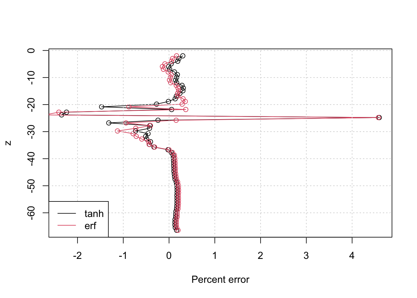
Calculating the root mean square differences is one way to see which one fits “better” (as Twitter wanted to know):
| tanh_rms | erf_rms |
|---|---|
| 0.0281296 | 0.0292661 |
Looks like the \(\tanh\) just edges out the win!2
Post Script
I found the fact that these two functions are very similar to each other interesting, and so apparently did someone who asked about it on the Math Stack Exchange back in 2016. There are some nice details there, but the main point is that the first two terms in the Taylor series expansions are identical, meaning that the difference between them for small values is \(O(x^5)\). A direct comparison of the two functions gives:
erf <- Vectorize(function(x) integrate( function(t) {2/sqrt(pi) * exp(-t^2)}, 0, x)$value)
x <- seq(-10, 10, 0.01)
par(mfrow=c(2, 1), mar=c(3, 3, 0.5, 1), mgp=c(2, 1, 0))
plot(x, 2/sqrt(pi)*tanh(x), type='l', xlab='')
lines(x, erf(x), col=2)
grid()
plot(x, 2/sqrt(pi)*tanh(x) - erf(x), type='l')
grid()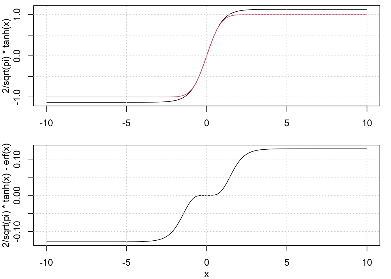
Martini, Kim I., David J. Murphy, Raymond W. Schmitt, and Nordeen G. Larson. “Corrections for Pumped SBE 41CP CTDs Determined from Stratified Tank Experiments.” Journal of Atmospheric and Oceanic Technology 36, no. 4 (April 2019): 733–44. https://doi.org/10.1175/JTECH-D-18-0050.1↩︎
But not really, since those numbers are likely statistically indistinguishable given the variation.↩︎