Functions to model ocean interfaces

2021-01-24 in OCEANOGRAPHY • R
ctd data statistics
3 min read

A while ago, I found a beautiful CTD profile in our AZMP data archive, that was a nearly perfect fit to one of my favourite functions, the \(\tanh\) function: A perfect CTD profile.

library(oce)
ctd <- read.oce('D19002034.ODF')

## Warning in read.odf(file = file, columns = columns, exclude = exclude, debug =
## debug - : "CRAT_01" should be unitless, but the file states the unit as "S/m" so
## that is retained in the object metadata. This will likely cause problems. See ?
## read.odf for an example of rectifying this unit error.

par(mfrow=c(1, 2))
plot(ctd, which=1, type='l')
plot(ctd, which=5)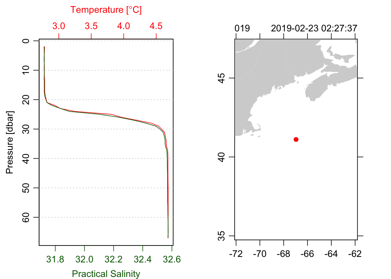

Following a Twitter chat with my good friend and expert oceanographer Kim Martini, I re-learned about the “Error Function”, often abbreviated as erf(), which she uses to model diffusive interfaces. Intriqued, I decided to write up my explorations here.

From Wikipedia, we can see that erf() (AKA the Gauss error function) is the integral of something much like a Gaussian:

\[ erf(z) = \frac{2}{\sqrt{\pi}} \int_0^z e^{-t^2}\,dt \]

Because it is an integral, we can define the gradient of the field for which we want an interface (i.e. the “stratification”, if we are thinking about density profiles) and then simply integrate it to get the profile. For example:

z <- seq(-3, 3, length.out=100)
# thickness of the interface, defined as a standard deviation
sigma <- 0.5 
grad <- 1/(sigma * sqrt(2*pi)) * exp(-1/2 * z^2/sigma^2)
par(mfrow=c(2, 1), mar=c(3.5, 3.5, 0.5, 3))
plot(z, grad, type='l')
profile <- integrateTrapezoid(z, grad, 'cA')
plot(z, profile, type='l')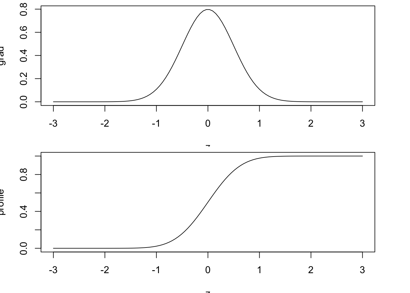

For that example, I used a numerical integration function from the oce package that uses the canonical “trapezoidal rule”. Easy to use, but not all that practical if we want a generic function, as it is an approximation whose accuracy depends on the resolution of the variable of integration (i.e. z).

Another approach is to take advantage of the numerical integration that is built-in to R, through the integrate() function. integrate() takes as an argument a function which defines the integrand, so it can be used to approximate the integral in a much more programmatic way.

First, we define a function that returns a Gaussian:

gaussian <- function(z, sigma=1) 1/(sigma * sqrt(2*pi)) * exp(-1/2 * z^2/sigma^2)
plot(z, gaussian(z))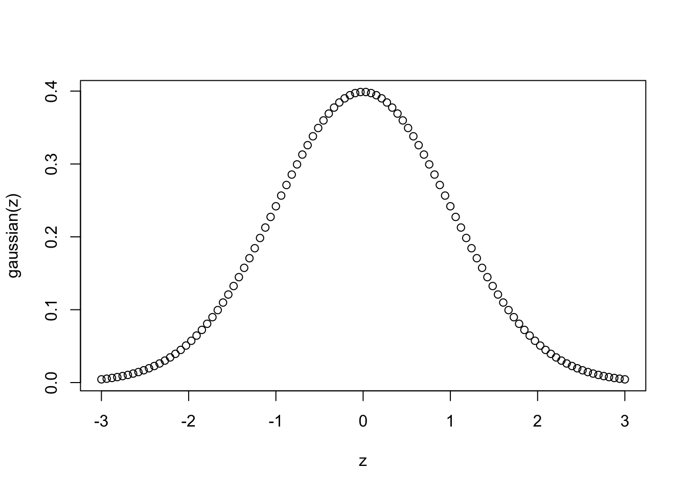

To integrate this, we can do:

integrate(gaussian, 0, 1, sigma)

## 0.4772499 with absolute error < 5.3e-15

but that gives us a single value, whereas what we want is a function that returns the integral much like our trapezoidal example above. To do this we write the integrate() call into a traditional R function, but we also use the Vectorize() function to turn the result into a vector:

int <- Vectorize(function(z, sigma=1) integrate(gaussian, 0, z, sigma)$value)
par(mfrow=c(2, 1), mar=c(3.5, 3.5, 0.5, 3)) 
plot(z, gaussian(z), type='l')
plot(z, int(z), type='l')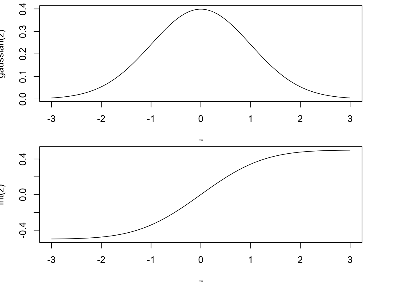

Now, putting it all together, and making some tweaks to account for the fact that we want the interface to be centered at a particular depth zi, and we want the interface to transition from a value in the upper layer (c1) to the value in the lower layer (c2), we get as below:

interface <- function(z, zi, c1, c2, sigma=1) {
    gaussian <- function(z, sigma) 1/(sigma * sqrt(2*pi)) * exp(-1/2 * z^2/sigma^2)
    int <- Vectorize(function(z, sigma=1) integrate(gaussian, 0, z, sigma)$value)
    0.5*(c1 + c2) + (c1 - c2) * int(z - zi, sigma)
}

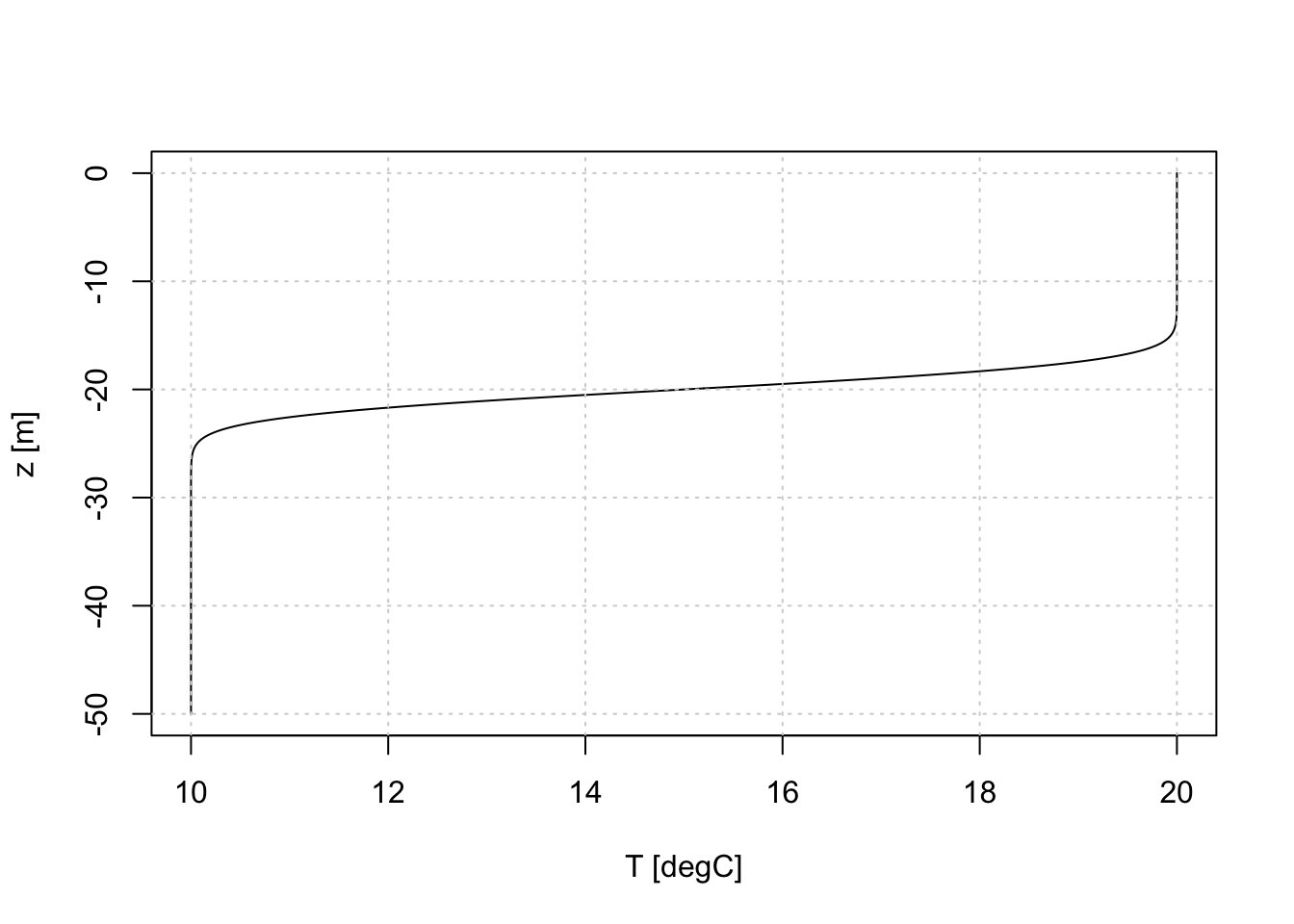
Trying it out on a more realistic scenario, say for a temperature profile in a 50m deep ocean, with 20 degrees C at the surface and 10 degrees C at the bottom, for an interface 2m thick centred at \(z=-20\)m, we get:

z <- seq(0, -50, -0.1)
plot(interface(z, zi=-20, c1=20, c2=10, sigma=2), z, type='l',
     xlab='T [degC]', ylab='z [m]')
grid()

Related Articles